Neural network training relies on our ability to find “good” minimizers of highly non-convex loss functions. It is well known that certain network architecture designs (e.g., skip connections) produce loss functions that train easier, and well-chosen training parameters (batch size, learning rate, optimizer) produce minimizers that generalize better. However, the reasons for these differences, and their effects on the underlying loss landscape, are not well understood.
In this paper, we explore the structure of neural loss functions, and the effect of loss landscapes on generalization, using a range of visualization methods. First, we introduce a simple “filter normalization” method that helps us visualize loss function curvature, and make meaningful side-by-side comparisons between loss functions. Using this method, we explore how network architecture affects the loss landscape, and how training parameters affect the shape of minimizers.
The original article, and an implementation using the PyTorch library, are available here.
Visualizing the Loss Landscape of Neural Nets
Implementation on Github
A 3D interactive visualizer, and a detailed blog post describing visualization methods, has been provided by Ankur Mohan.
Finally, we suggest you visit losslandscape.com to view stunning artistic renderings of neural loss landscapes.
Sample results
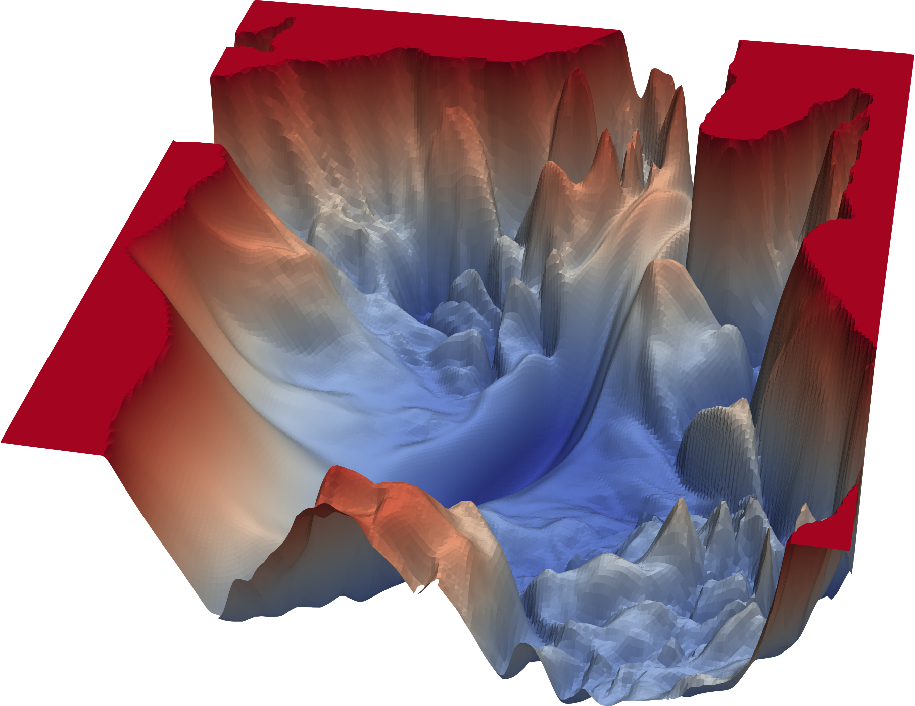
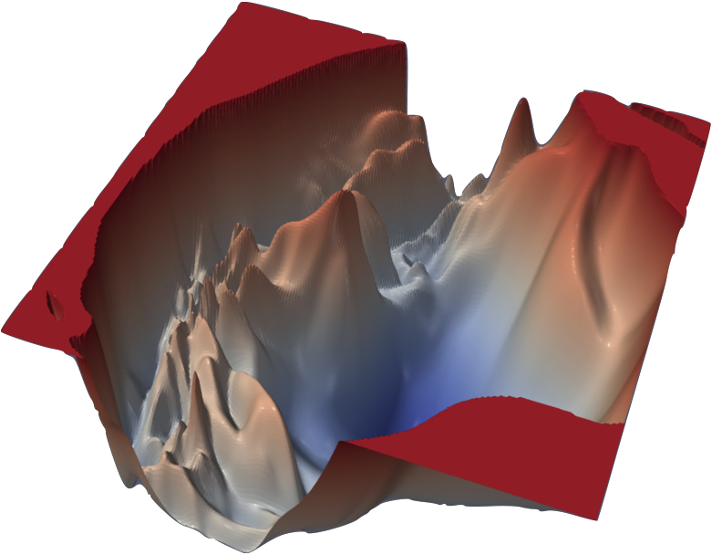
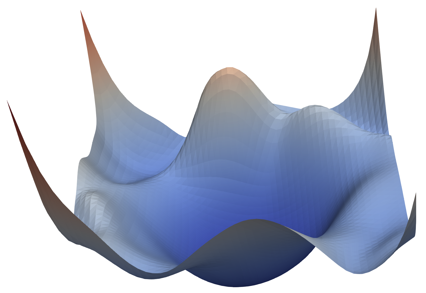
We find that network architecture has a dramatic effect on the loss landscape. Shallow networks have smooth landscapes populated by wide, convex regions. However, as networks become deeper, landscapes spontaneously become “chaotic” and highly non-convex, leading to poor training behavior. Certain network architecture designs, like skip connections and wide networks (many filters per layer), undergo this chaotic transition at much more extreme depths, enabling the training the deep networks.
VGG-56
VGG-110
Renset-56
Densenet-121
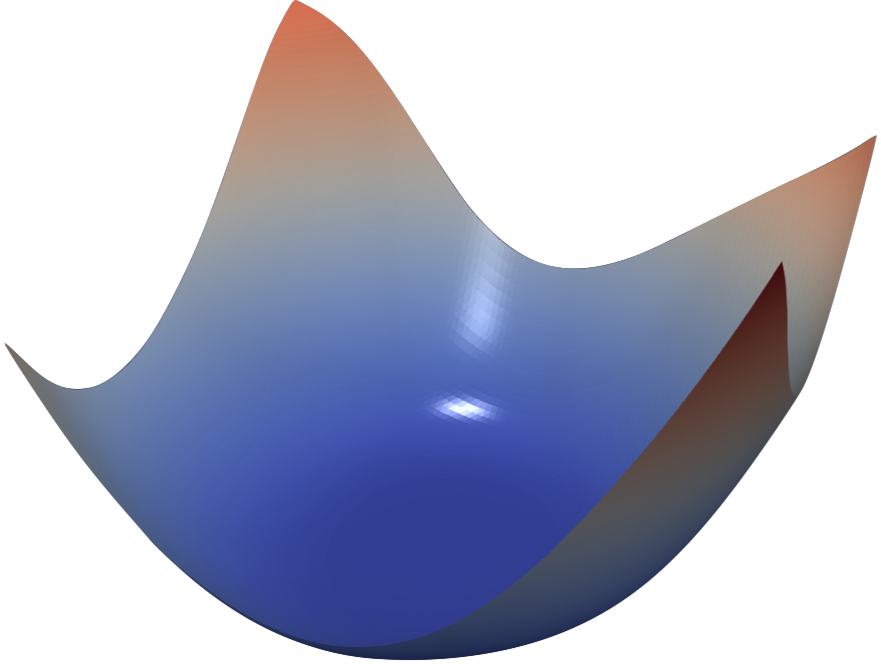
Neural loss functions with and without skip connections. The top row depicts the loss function of a 56-layer and 110-layer net using the CIFAR-10 dataset, without residual connections. The bottom row depicts two skip connection architectures. We have Resnet-56 (identical to VGG-56, except with residual connections), and Densenet (which has a very elaborate set of skip connections). Skip connections cause a dramatic "convexification" of the loss landscape.
Other contributions
This paper also explores “sharp” vs “flat” minimizers. We show that conventional visualization methods fail to capture the endogenous “sharpness” of minimizers, and that the proposed filter-normalization method provides a reliable way of visualizing sharpness that correlates well with generalization error.
We also study the effect of different optimizers (SGD vs ADAM) and training parameters (momentum, learning rates) on the geometry of minimizers. Using visualization methods, we plot the trajectories taken by different optimizers on top of the underlying loss function, and explore how learning rate schedules affect convergence behavior.
Acknowledgements
![]() This work was made possible by the generous support of the Office of Naval research, and was done is collaboration with the United Stated Naval Academy.
This work was made possible by the generous support of the Office of Naval research, and was done is collaboration with the United Stated Naval Academy.